Recommender Systems - Content Based
Prerequisites
- python environment with
numpyandpandasinstalled - dataset files
attributes.csvandreviews.csvlocated here
Description
This post provides a basic introduction to content based filtering and walks through an example that shows how to build a simple content based recommender that recommends documents based on user preferences.
What is Content Based Filtering?
Content based filtering is one of the main categories of recommender systems. It recommends items based on attributes - how similar two items are based on their attributes.
For example take a movie with a single attribute - starring actor
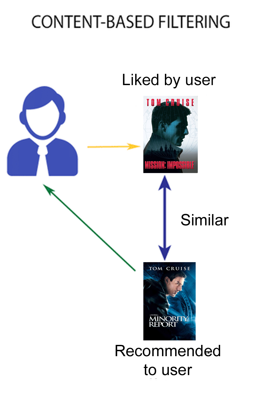
The assumption being made here is because the movies share a starring actor they are considered similar. Thus a movie that is similar to Mission Impossible is Minority Report, which gets recommended to the user.
Generally, if a user expresses a preference for an item, the user may like similar items.
The end result of content filtering is to build up a profile of things a user likes and doesn’t like and use that to predict their liking of other items.
Dataset
The data set consists of two files.
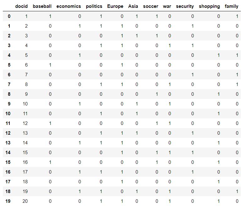
attributes.csv is a list of documents (rows), they could be anything like news articles or movie overviews. The columsn replresent a list of attributes - the attributes can be a list of keywords for movies, or even an entire corpus of words for a set of articles. The cells contain a count of value 0 or 1 which represents if the attribute is present in the corresponsding document, 0 not present, and 1 is present.
This is also called an Item Content Matrix (ICM).
reviews.csv is a list of preferences for each document for several users. The rows again are the documents, and the columns are the users. Each cell contains a rating value of -1 for dislike, 0 for no rating, and 1 for like. We can assume that this is a snapshot of user preferences at some point in time and as time goes on users one and two will like or dislike new articles.
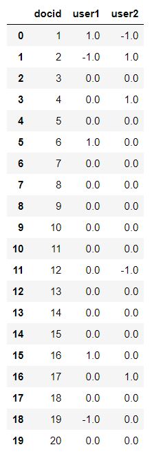
Reviews can be joined to the attributes by the docid column.
Building the recommender
Loading libraries
We will need to import math, pandas, and numpy
import math
import numpy as np
import pandas as pd
Loading the data
We will load the data set into two separate dataframes, one for attributes, and one for reviews.
# load the attributes
attributes_df = pd.read_csv(r'attributes.csv')

# there two unamed empty columns at the end so we have to drop those first
attributes_df = attributes_df.drop(attributes_df.columns[11:13],axis=1)

# load the reviews - notice that we have to remove the NaN values by replacing them with zeros
ratings_df = pd.read_csv(r'ratings.csv').fillna(0)
Convert to numpy arrays
attributes_np = attributes_df.drop(attributes_df.columns[0],axis=1).to_numpy()
reviews_np = ratings_df.drop(ratings_df.columns[0],axis=1).to_numpy()
User Profiles
Create basic user profiles - multiply each user ratings row by the attributes row for each document, then once complete sum each column
profile1 = []
profile2 = []
for i in range(0,10):
    column = attributes_np[:,i]
    product1 = np.dot(column,reviews_np.T[0])
    product2 = np.dot(column,reviews_np.T[1])
    profile1.append(product1)
    profile2.append(product2)

profile1_np = np.array(profile1)
profile2_np = np.array(profile2)
Predictions
Compute the predicted score for each user for each document (a simple dot-product).
user1_prediction = [np.dot(i,profile1_np) for i in attributes_np]
user2_prediction = [np.dot(i,profile2_np) for i in attributes_np]
This basic model is consistent with the users’ ratings – it predicts liking for all the positive documents and disliking for all the negative ones.
However an article that had many attributes checked could have more influence on the overall profile than one that had only a few, So in the next step we will try and remove this bias in the model due to counting attribute heavy documents too much.
Normalization
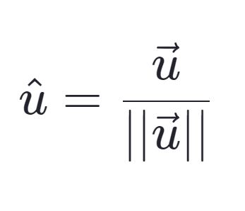
Normalize each row of the attributes matrix to be a unit length vector. Do this by dividing each value in the row by the magnitude of the vector. THe magnitude is calcualted by taking the square of each item, summing them up and then taking the square root of that value.
The formula for this is as follows
# create a copy of the proginal matrix
attributes_normalized = attributes_np.copy().astype('float64')

# normalize
for i in range(len(attributes_normalized)):
    num = np.sum(attributes_normalized[i])
    attributes_normalized[i] = attributes_normalized[i]/math.sqrt(num)

# calculate the new user profiles
profile1_normalized = []
profile2_normalized = []
for i in range(0,10):
    column = attributes_normalized[:,i]
    product1 = np.dot(column,reviews_np.T[0])
    product2 = np.dot(column,reviews_np.T[1])
    profile1_normalized.append(product1)
    profile2_normalized.append(product2)

# caclulate the predictions
user1_prediction_normalized = [np.dot(i,profile1_normalized) for i in attributes_normalized]
user2_prediction_normalized = [np.dot(i,profile2_normalized) for i in attributes_normalized]
Using IDF to account for frequencies of attributes
Now we will account for the fact that the content attributes have vastly different frequencies.
Inverse Document Frequency (IDF) is a weight indicating how commonly a word is used. The more frequent its usage across documents, the lower its score and the less important it becomes. In essense it is a measure of ‘rareness’ of a term.
For example, the word the appears in almost all English texts and thus has a very low IDF score. In contrast, if you take the word baseball it is not used as widely as the word the so it would have a higher IDF score than the making it of more importance.
The most common formula for this is as follows, where n is the number of documents and dfj is the document frquency of attribute j across the n documents.
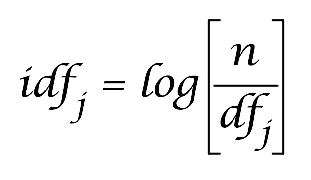
In this case we will not use this formula exactly due to the small dataset size. Instead we will simply use the inverse of document frequency - 1/df, so that we can see differences in the results more easily.
# calculate 1/df
documentfrequency = attributes_np.sum(axis = 0)
documentfrequency.astype('float64')
inverse_df = 1/documentfrequency

# get the predictions
# multiply each term IDF by document term , then take sum of the product (dot product) of (document vector X IDF) * profile
user1_prediction_idf = [sum(i*inverse_df*profile1_normalized) for i in attributes_normalized]
user2_prediction_idf = [sum(i*inverse_df*profile2_normalized) for i in attributes_normalized]
Results
Lets take a look at some predictions.
print(user2_prediction[5], user2_prediction_idf[5])For Document 6 user 2 preference is now negative -0.08469536214019152 wheras before it was positive 1.0. This changed because IDF reduced the weight of the more frequent term ‘Europe’
Let’s print out the predictions for user 1 before and after using IDF, and sort them from most to least favorite.
# top documents for user 1 before using IDF
simple = pd.DataFrame()
simple['before'] = user2_prediction
simple['docid'] = attributes_df['docid']
sorted_simple_df = simple.sort_values(by='before', ascending=False)

# top documents for user 1 after using IDF
after_df = pd.DataFrame()
after_df['after'] = user2_prediction_idf
after_df['docid'] = attributes_df['docid']
sorted_after_df = after_df.sort_values(by='after', ascending=False)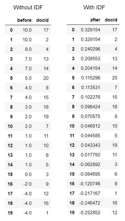
The top 5 documents haven’t changed in ranking. We can see more differences as we move down the rankings. For example lets look at a document that user never read before and thus never rated - Document 19. Before it was ranked as 9th place with a preference rating of 2.0, but now it moves down to 12th place with a rating of 0.04.
It contains attributes with document frequencies
- economics = 10
- politics = 11
- Asia = 6
- war = 7
- family = 5
User 1 likes documents 1 (with attributes poitics, Asia, and family), document 6 (no attributes), and document 16 (no attributes)
Of all the attributes in common with the liked documents, politics, Asia and family remain. Politics having such a high document frequency is now given less weight. This could explain why the ranking has gone down somewhat.
Conclusions
We can see that the very basic predictions in the first step provides somewhat reasonable predictions, however the predictions are biased toward documents that have more attributes.
Using normalization and Inverse Document Frequency we are able to balance the weights of the attributes depending on their frequency of appearance in the documents.
This concept can be applied to any number n of items and can be used to find out which items a user will like the most. Therefore, as new items such as articles or movies are added, recommendations can be made to a user based on preference for items which were seen already.
Source Code
References
Introduction to Recommender Systems: Non-Personalized and Content-Based
by University of Minnesota
Salvatore S. © 2020